How to Evaluate Associated Gas Power Generation ROI: A Gas Volume & Equipment Sizing Guide

Most oilfield operators already know associated gas-to-power works. The real question is: will it work for my specific field, at my specific gas volume, with my specific cost structure?

This guide answers that question — not with marketing promises, but with a gas-volume-driven ROI framework that lets you calculate your own payback number. If you’ve already read our analysis of the flaring dilemma and our breakdown of high-H₂S handling technology, this is the next step: the numbers that determine whether the investment pencils out.

The ROI Equation: Three Variables That Determine Your Payback

Associated gas power generation economics boil down to three inputs that every field engineer can measure:

1. Daily flared gas volume (m³/day) — the fuel supply. More gas = more potential generation = faster payback.
2. Current delivered power cost ($/kWh) — what you’re paying today for diesel generation, including fuel, trucking logistics, generator rental, and maintenance.
3. Field remaining life (years) — how long the asset will produce. Units are redeployable, but the upfront investment needs enough runway to pay back.

Everything else — H₂S concentration, gas pressure, ambient temperature — affects the feasibility of gas-to-power, not the core economic logic. These are engineering problems with proven solutions. The only question that matters for ROI is whether the gas volume justifies the equipment size.

Gas Volume Tiers: How Much You Flare Determines Your Payback

The relationship between gas volume and payback is non-linear. Below is a tiered framework based on field operating data from Xinjiang and Qinghai deployments:

Gas Volume Tier	Flared Gas (m³/day)	Usable Power (kW)	Recommended Unit	Indicative Payback
Tier 1 — Minimum Viable	25K–50K	200–400	JTF-200 / 400	14–18 months*
Tier 2 — Standard	50K–150K	400–1,000	JTF-400 / 600 / 800	8–14 months
Tier 3 — Sweet Spot	150K–500K	1,000–3,000	2–3 × JTF-1000 (modular)	6–10 months
Tier 4 — Large-Scale	500K+	3,000+	Multi-unit cluster	5–8 months

*Tier 1 payback assumes diesel cost ≥ $0.25/kWh delivered. Below this, the economics weaken — a diesel-gas hybrid with gas providing baseload and diesel for peaks may be more practical.

The sweet spot is clear: fields flaring 150K–500K m³/day with delivered diesel costs above $0.20/kWh hit payback in under 10 months. This is not a marginal improvement — it’s a step change in operating cost structure.

Why Gas Volume Matters More Than Gas Quality

Associated gas composition — H₂S content, BTU variability, moisture — determines the engineering cost of gas-to-power, not the economic viability. H₂S up to 2,000 mg/Nm³ is handled with corrosion-resistant materials in the fuel train, as demonstrated in Xinjiang for 5+ years. The additional capex for sour gas handling is $100K–300K — meaningful, but absorbed within the 6–14 month payback window.

What kills the economics is not difficult gas — it’s insufficient gas. A field flaring 10K m³/day simply doesn’t produce enough fuel to generate meaningful power. The 25K m³/day threshold is the practical minimum for a standalone 200 kW unit running at 85% capacity factor.

Equipment Selection Decision Tree

The JTF Series spans six power ratings (100 / 200 / 400 / 600 / 800 / 1,000 kW), all modular and interconnectable. Choosing the right unit — or combination of units — is a function of three parameters:

Field Condition	Gas Volume (m³/day)	Recommendation
Single well pad, low volume	25K–50K	1 × JTF-200 or JTF-400
Production facility, steady flow	50K–150K	1 × JTF-600 or JTF-800
Central processing, multiple wells	150K–300K	2 × JTF-600 or 1 × JTF-1000 + JTF-400
Large field, central facility	300K–500K	2–3 × JTF-1000 modular cluster
Seasonal fluctuation ±30%	Variable	Modular pair (e.g., 2 × 400 kW), take one offline in low season

The modular architecture is central to the economic model. A 1,000 kW unit is not stranded when a field depletes — it is disconnected, trucked to the next location, and recommissioned in 2–4 weeks. This redeployability transforms the asset from a sunk cost into a movable capital item that follows production across a basin.

Complete Flare Gas Recovery Architecture: From Wellhead to Power Bus

The containerized CHP unit is the most visible component — but it’s only one link in the flare gas recovery chain. A complete system consists of five stages:

Stage	Component	What It Does	Why It Matters for ROI
1. Gas Capture	Wellhead separator → knockout drum	Separates associated gas from crude and water at the production manifold	Zero additional infrastructure if the field already has separation — most do
2. Fuel Conditioning	Filtration + moisture removal + H₂S-compatible materials	Removes particulates, condensate droplets, and handles H₂S up to 2,000 mg/Nm³ without sweetening	No separate amine plant required for standard sour gas — capex stays at $600K/MW
3. Power Generation	Spark-ignition gas engine + PM alternator	Converts 38–42% of fuel energy to electricity (ISO 3046); smart load tracking adjusts output to demand	Electricity eliminates diesel purchase — the single largest cost reduction
4. Heat Recovery	Jacket water + exhaust heat exchangers	Captures 43–47% of fuel energy as usable heat for crude pre-heating or facility climate control	Displaces heater-treater fuel; total system efficiency ≥85%
5. Balance of Plant	Power distribution panel, SCADA telemetry, backup tie-in	Connects to site power bus; remote monitor/control via 4G/5G; existing diesel generators retained for backup only	Unmanned operation, no additional headcount; existing diesel becomes standby insurance

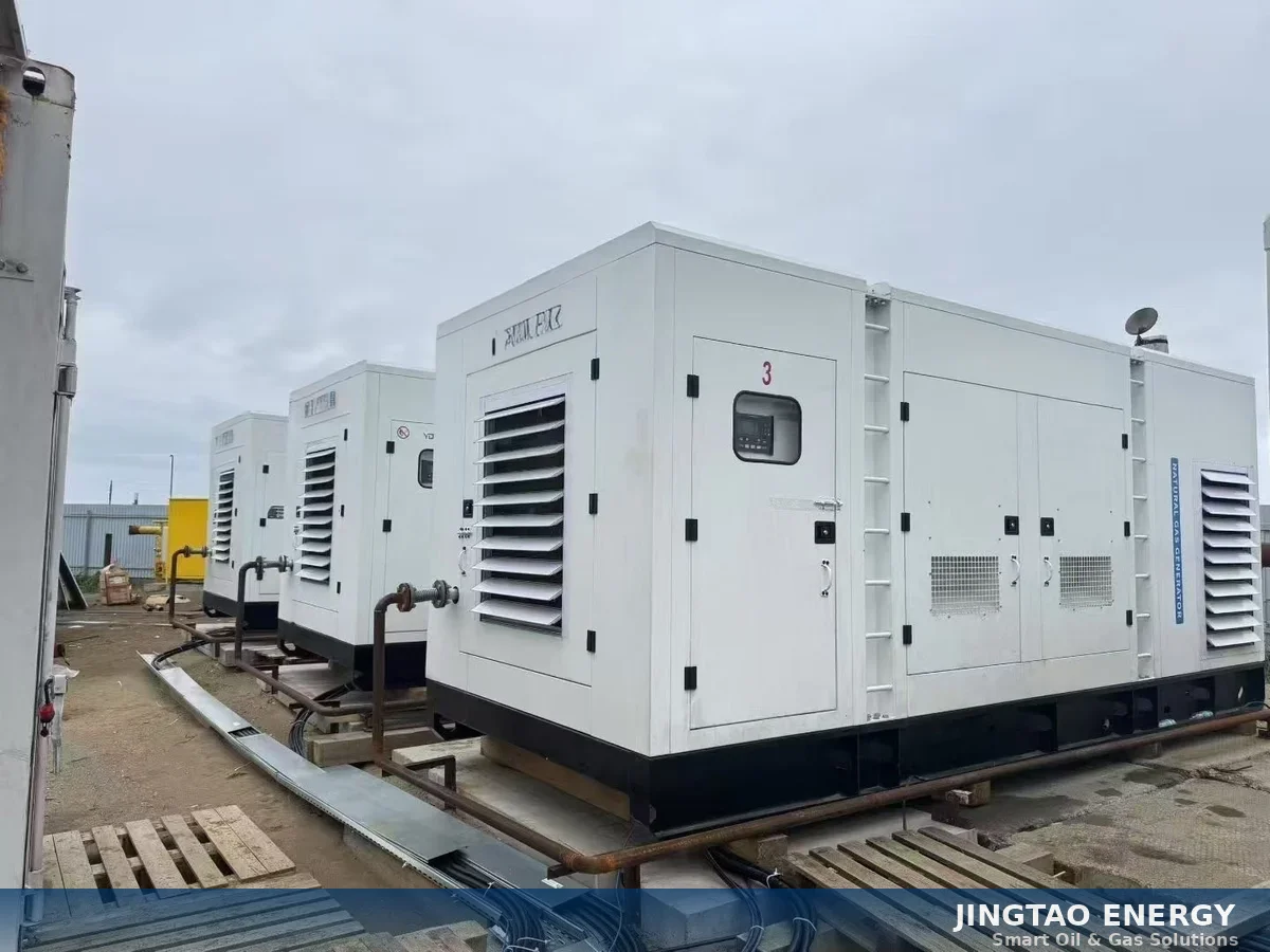
The complete architecture ships as a single ISO container lift — 20-foot for units up to 400 kW, 40-foot for 600–1,000 kW. Site preparation requires a concrete pad, gas line connection, and power bus tie-in. Total deployment from contract signature to first power: approximately 3 months (8–12 weeks production + 2–4 weeks commissioning).

Real-World ROI: What the Numbers Look Like in the Field

Xinjiang Oilfield — Tier 3 Sweet Spot

A remote production facility in China’s Xinjiang basin: +50°C summers, 2,000 ppm H₂S in the gas stream, no grid access. The operator was running diesel generators 24/7 at delivered fuel costs exceeding $0.30/kWh. Flared gas volume: approximately 180,000 m³/day — firmly in Tier 3.

They deployed a containerized 1 MW JTF-1000 unit running on raw wellhead gas. No pre-treatment. No sweetening. The unit powered ESPs, sucker rod pumps, and facility loads.

• Payback achieved: 14 months
• Status after 5 years: Continuous operation, standard maintenance intervals
• Diesel consumption: Reduced to zero for base load; existing generators retained for maintenance shutdowns only

Qinghai Oilfield — Cold Climate, Standard Economics

The same system architecture operating at −30°C winter ambient — proving the temperature envelope is not a constraint. Payback profile comparable to Xinjiang, with slightly higher maintenance cost for cold-weather oil grades.

Both deployments share the same economic driver: the fuel is free because it was being flared anyway. The only costs are the equipment (capex) and maintenance (opex at $0.008–0.012/kWh).

Why 2026 Is the Decision Window

The regulatory trajectory is clear, and the financial penalties for inaction are compounding:

• World Bank Zero Routine Flaring by 2030: Over 30 governments have committed. Operators without a flare reduction plan will face license renewal challenges.
• Nigeria: Gas flaring penalty increased from $2.00 to $3.50/Mcf in 2025. For a field flaring 200,000 m³/day (~7 MMcf), that’s approximately $8.9M/year in penalties.
• EU CBAM: The Carbon Border Adjustment Mechanism is operational and expanding. Carbon intensity of exported crude is becoming a commercial differentiator.
• IFC/Multilateral Development Banks: Now require flare reduction commitments as a condition of oil and gas project financing.

The arithmetic is straightforward: deploy gas-to-power at $600K/MW with 6–14 month payback, or continue paying diesel fuel costs plus escalating regulatory penalties. The window to deploy before compliance costs harden further is 2026–2027.

Frequently Asked Questions

How do I calculate the exact gas volume needed for a specific power requirement?

Use the rule of thumb: approximately 100,000 m³/day of standard associated gas (600–1,200 BTU/scf) yields roughly 1 MW of electrical output at 38–40% engine efficiency. For a 500 kW requirement, you need approximately 50,000 m³/day. For 2 MW, approximately 200,000 m³/day. A site-specific gas composition analysis refines this estimate — methane content, BTU value, and inert fraction all affect the conversion ratio. We recommend a 30-day flow measurement before final equipment sizing.

What happens to payback if my gas volume fluctuates seasonally?

Seasonal fluctuation is the most common variable that stretches payback beyond the baseline 6–14 month range. If gas volume drops 30%+ during certain months, a modular approach (two smaller units instead of one large one) preserves economics — you run one unit at high load during low-flow months rather than one large unit at inefficient partial load. When modeling ROI, assume 85–90% annual capacity factor, not 100%. At 85% capacity factor, Tier 2 payback extends from ~8 months to ~11 months — still well within the investment case.

Can I run gas-to-power and still keep my diesel generators?

Yes — and this is the recommended approach. Gas-to-power serves base load; existing diesel generators are retained as backup for maintenance windows, unexpected gas interruptions, or peak demand above gas-to-power capacity. This hybrid configuration eliminates the risk perception of “going all-in on gas.” The diesel fleet becomes an insurance policy rather than a daily operating expense, with fuel consumption dropping 85–95%.

What is the minimum field life required to justify gas-to-power?

The minimum field remaining life should exceed the payback period by at least 6 months. For a Tier 2 field with 10-month payback, you need 16+ months of remaining production. However, the redeployability of containerized units changes this calculus — if you have a follow-on field in the same basin, the unit moves. In that case, the economic horizon extends beyond any single field’s depletion date. Operators managing multiple fields in the same concession should evaluate gas-to-power at the portfolio level, not the individual field level.

How does heat recovery affect the ROI calculation?

Heat recovery from jacket water and exhaust — capturing 43–47% of fuel energy as usable thermal output — can cut payback by 2–4 months if the field has a year-round thermal load. Crude pre-heating for separation, heater-treater fuel displacement, and facility climate control are the most common uses. A field requiring 200 kW of thermal energy for crude heating that currently burns purchased fuel will see the CHP unit’s payback accelerate as that fuel purchase is eliminated. Fields without thermal demand still benefit — but the payback is driven entirely by electricity displacement, typically landing at the upper end of the 6–14 month range.

What external certifications or standards apply to these units?

JTF Series units comply with EPA Tier 2 and EU Stage IIIA emissions standards as standard, with optional SCR upgrade to Tier 4. Electrical output meets IEC 60034 for generator performance. The containerized design follows ISO 668 for standard shipping container dimensions, enabling global freight by road, rail, or sea. Hazardous area certifications are available for Zone 2 installations.

Technical Data Sheet — JTF Series Smart Gas Generator Sets

Parameter	Specification
Power Range	100 / 200 / 400 / 600 / 800 / 1,000 kW (modular, parallel-capable)
Electrical Efficiency	38–42% (ISO 3046 conditions)
Total CHP Efficiency	≥85% (electrical + thermal recovery)
Fuel Types	Associated gas / flare gas / natural gas / biogas
H₂S Tolerance (Standard)	≤200 mg/Nm³
H₂S Tolerance (Upgraded)	≤2,000 mg/Nm³ — field-validated, 5 years continuous (Xinjiang)
Inlet Gas Pressure	5–50 kPa (0.05–0.5 bar) at engine inlet
Output Voltage	400V / 480V 3-phase, 50/60 Hz (customizable)
Emissions Compliance	EPA Tier 2 / EU Stage IIIA (standard); SCR upgrade to Tier 4 available
Enclosure	Containerized skid (20 ft ≤400 kW, 40 ft ≥600 kW), weatherproof, sound-attenuated
Installed Cost	~$600,000/MW (vs $1.5–2.5M/MW conventional gas plant)
Payback Period	6–14 months (fuel-free operation, field-validated)
Delivery Timeline	8–12 weeks production + 2–4 weeks site commissioning
Annual Maintenance Cost	$0.008–0.012/kWh
Operating Temperature Range	−30°C to +50°C (field-validated: Qinghai −30°C, Xinjiang +50°C)
Control System	Smart load tracking — auto-adjusts to power demand and gas supply pressure

Data from field operating records (Xinjiang and Qinghai oilfields) and manufacturer specifications. Individual project economics depend on gas composition, local diesel cost, and thermal load profile. Contact us for a site-specific ROI analysis.

---

Ready to calculate your field’s ROI?

→ JTF Series Smart Gas Generator Sets — complete specifications and deployment architecture
→ CHP Economics Deep-Dive — unit economics, CAPEX comparison, and Central Asia 6-unit case study
→ The Flaring Dilemma — why 2026 is the year operators can no longer afford to flare
→ Request a Site-Specific Payback Analysis — share your gas volume and power cost, we’ll return a customized ROI model