How to Evaluate Wax Prevention Cost: 5 Drivers That Decide Electromagnetic Wax Control ROI

Two wells with the same wax problem, the same rod-pump completion and the same equipment scope can produce two completely different payback outcomes — and neither of them is decided by the unit itself. What decides it is the intervention ledger, the well’s screening profile and how the operator has been budgeting wax control until now.

1. Why “Cost Per Treatment” Is the Wrong Denominator

Wax management is normally budgeted as a treatment line: inhibitor volume per month, hot-oil circulation per quarter, mechanical scraping runs as required. That accounting convention creates a specific bias — it makes prevention look expensive, because it compares a one-off capital installation against a per-job service rate that has already been normalized into the operating budget. It is not a like-for-like comparison, and it is the most common reason electromagnetic (EM) wax prevention gets rejected in a first screening.

The right denominator is the total cost of keeping flow open across a defined production horizon — one year, five years, ten years — including the costs that never appear on the treatment line at all: deferred barrels while the well is shut in, workover-unit mobilization in remote fields, and personnel exposure on every intervention. A 2023 review in *Energies* on the economics of waxy crude records that wax deposition has been estimated to affect 85% of global oil production, while cautioning that the figure cannot be precisely quantified [1]. That uncertainty is precisely why a well-by-well model beats a benchmark number pulled from someone else’s field.

The reason the two options are so often mis-compared comes down to shape. Reactive wax control is a stream of small recurring costs that never amortize and never end. EM prevention is one capital event followed by near-zero operating cost over a long service life. A five-year bill comparison has been covered in detail in our lifecycle cost analysis of electromagnetic and chemical wax control — the purpose here is different: to show which variables actually move that bill, so you can build the number for your own wells instead of borrowing ours.

Three questions decide whether a wax-control investment ever clears a capital review: how often does this well currently stop producing, what does each stop cost in full, and what is the remaining producing life over which to amortize the fix. Everything below is a way of answering those three questions with data you already have.

2. The Five Cost Drivers of Electromagnetic Wax Prevention

Across the field data behind more than 800 installed units, the commercial case resolves into five variables. They are not equally weighted — the first two set the ceiling, the last three decide whether the ceiling is reachable.

Cost driver	What it changes in the model	How to estimate it	Where the case is strongest
1. Baseline intervention frequency	Size of the avoided-cost pool — the multiplier on everything else	12 months of cleaning / scraping / hot-oil / workover records, counted by type	High-wax wells on weekly-to-monthly intervention cycles
2. Lift method and well type	Whether the device can act on the produced fluid at all	Completion records: rod pump, flowing, gas lift, ESP conversion history	Continuous rod-pump production with steady liquid rate
3. Wax and fluid severity	How much of the physical effect reaches the flowline	Wax appearance temperature, wax content, asphaltene fraction, water cut	Moderate-to-high wax, water cut below 30%
4. Flowline geometry, site and certification envelope	Capital scope and installation window	Line bore, pressure class, hazardous-area classification, available power	Standard land wellheads; offshore and Ex-rated configurations add scope
5. Intervention logistics and exposure	The hidden layers of the avoided cost	Distance to service base, crew mobilizations per year, safety exposure per trip	Remote fields where mobilization dominates the intervention cost

Driver 2 is a screen, not a score. A well that fails it cannot be rescued by a favourable frequency figure, however attractive the arithmetic looks on a spreadsheet.

3. Driver 1 — Baseline Intervention Frequency: the Multiplier on Everything

Frequency is the multiplier in every wax-control ROI model. A well on a seven-day scraping cycle is competing against dozens of interventions per year, so the avoided-cost pool is large and one installation has plenty to work against. A well that is hot-oiled once a year cannot justify the same capital outlay on avoided intervention cost alone — and pretending otherwise wastes the operator’s time as well as ours. Our field data on workover and cleaning frequency shows the two ends of that range in practice.

Intervention frequency runs high where crude is waxy, water cut is low, the surface flowline is long, ambient temperature swings hard between seasons, and the field already has a history of wax-related shutdowns. It runs low in lighter-crude fields with short flowlines — which is the honest reason payback in parts of the Middle East is longer than the same scope in a high-wax onshore field in Asia.

Build the baseline from the maintenance ledger, not from memory. Count each intervention type separately and note which ones were driven by wax rather than by unrelated failures:

Chemical injection or inhibitor top-up visits

Hot-oil or hot-water circulation jobs and the hours of deferred production attached to each

Mechanical scraping or pigging runs, including the crew mobilized

Wax-related workovers — the expensive tail, and the one that never gets its own budget line

An estimate assembled from memory inherits its error directly into the model. A single season of records is usually enough to see the pattern; a full year is better because it captures the winter peak.

4. Driver 2 — Lift Method and Well Type: the Screen That Decides the Case

EM wax prevention acts on produced fluid as it passes through a controlled low-frequency magnetic field in the wellhead flowline. That requires continuous liquid flow through the device and enough residence time for the field to interact with the stream. Rod-pump wells satisfy both conditions and make up the overwhelming majority of the installed fleet.

Where the method weakens, it weakens because the physics changes — not because the hardware is at fault. In flowing and gas-lift completions the gas phase interrupts the field’s interaction with the liquid, and the treatment effect degrades sharply. In wells already converted to an ESP, or producing at a liquid rate below the device’s design envelope, the completion itself has changed and the economics have to be rebuilt from scratch.

Well profile	Screen result	Why	What to do instead
Rod pump, steady liquid rate	Candidate	Continuous liquid flow through the flowline device; the dominant installed fleet profile	Run the frequency model
Flowing / natural flow	Screened out	Gas stream interrupts field interaction with the liquid phase	Evaluate chemical inhibition or flowline thermal management
Gas lift with high gas-liquid ratio	Screened out	Same interruption problem; residence time in a two-phase mix is unstable	Look at the completion’s wax-control options with the operator
High gas rate, low liquid	Screened out	Too little liquid throughput to carry a benefit	No EM case
ESP converted / energy deficient	Re-model	Completion change alters the whole production basis	Rebuild the model on the new completion before quoting
High water cut (above 30%)	Conditional	Viscosity benefit weakens; intervention avoidance carries the case	Anchor the model on avoided interventions, not drag reduction

Reading a screening table honestly is worth more in a capital review than a favourable single-well example. It also protects the operator: an installation on the wrong completion is an installation that will be decommissioned early and taken as evidence against the technology.

5. Driver 3 — Wax and Fluid Severity: How Much of the Effect Reaches the Flowline

Bench testing with Petroleum University established the physical envelope: a reduction in wax crystallization temperature of 3–5 °C, an increase in wax dissolution capacity by a factor of 5.5, action distance beyond 2,000 m in laboratory conditions, and magnetic hysteresis of more than 4 hours after the fluid leaves the field.

The commercial consequence sits in the viscosity figures. Below roughly 30% water cut, measured viscosity reduction runs 30–80%, which improves flow and lowers pumping load. Above 30% water cut it falls to roughly 20% — and some fields produce above 85% water. On those wells the drag-reduction benefit largely disappears from the model, so the case has to stand on avoided scraping, avoided chemical spend and avoided workovers instead. Same device, different business case.

External peer-reviewed work supports the mechanism rather than taking our word for it. An experimental study published in *RSC Advances* in 2024 reported that both high-intensity and high-frequency magnetic treatment reduced wax deposition mass and produced a long-term magnetic history effect [2]; earlier loop experiments published in *Advanced Materials Research* reported reductions in both oil viscosity and wax deposition rate after magnetic treatment [3]. The magnitude depends on crude composition, field strength and residence time — which is why severity, not device rating, is the number that belongs in the model.

Severity can also disqualify a well outright. Extreme paraffin systems with a very high wax appearance temperature and high asphaltene content defeat the method: a Tarim Basin field operating at a 52 °C wax appearance temperature with more than 10% asphaltene and twice-daily scraping is not an EM candidate under any configuration we build. Screening it out early is the honest answer.

6. Driver 4 — Flowline Geometry, Site Conditions and Certification Envelope

Capital scope is set by the installation environment, not by the treatment principle. Four items drive it:

Line bore and pressure class — DN50, DN80 and DN100 units are standard, with flowline pressure classes of 2.5, 4 and 6 MPa; larger bores and higher ratings are custom scope

Physical installation — unit mass is roughly 70 kg at DN50 and 90 kg at DN80, which generally calls for wellhead support, and installation takes a skilled crew two to three hours after the well is stopped and the flowline is opened for the cut-in

Power and environment — the unit draws 650 W on a 380 V supply (customizable), and the unit is designed to run hot, dissipating through cooling fins. It must never be insulated; in desert service the cooling package is extended

Classification and options — standard land units, marine-climate units for offshore platforms, and explosion-proof units for hazardous areas, plus optional RS485 remote monitoring for run status, current and temperature

The offshore configuration is the clearest example of why scope follows environment: a platform installation changes the housing, the certification and the logistics, which is a different piece of work from a land wellhead even though the treatment parameters are identical. Chemical-free wax control on an offshore platform covers that configuration in more detail.

One practical note: the device needs continuous electrical supply and no local network. It runs unattended, which is what keeps operating cost near zero — but the power source has to exist before it is scoped, not after.

7. Driver 5 — Intervention Logistics, Deferred Production and HSE Exposure

The treatment budget captures one layer of the reactive cost. The full cost of an intervention has four:

Direct intervention cost — crew, equipment, consumables and the treatment itself

Deferred production — barrels not produced while the well is shut in; rarely a budget line, always a real cost

Mobilization in remote fields — in fields far from the nearest service base, getting a crew and unit to location frequently exceeds the treatment cost itself

Exposure — every intervention puts people on location and tools downhole; fewer interventions means fewer opportunities for an incident

Cost layer	Reactive wax control (chemical / hot oil / scraping)	EM wax prevention	Modelling note
Equipment and materials	Recurring — consumables every cycle, indefinitely	One capital event; no consumables	The one line most models get right
Labour and crews	Scales with intervention frequency	Installation only; no routine attendance	Use fully loaded crew cost, not day rate
Deferred production	Recurs at every shutdown	One shutdown for the cut-in	Value the barrels; the layer most often omitted
Logistics away from base	Per mobilization, per cycle	One mobilization at installation	Dominant in remote fields
HSE exposure	Proportional to intervention count	Proportional to installation count	Reduced by frequency, not by unit price
Energy draw	Fuel for hot oil; pumping load	650 W per unit, continuous	Small, but include it — it is the whole OPEX

Two rows in that table are usually missing from a first-pass comparison: deferred production and logistics. Add them and the balance shifts toward prevention in high-frequency wells; leave them out and the reactive option looks cheaper than it is.

8. A Four-Step Payback Model You Can Defend in a Capital Review

The model does not need software. It needs four numbers that an operator already owns, plus one that only the supplier can scope.

Step	What you compute	What you need	What it tells you
1. Baseline cost	Annual intervention count × fully loaded cost per intervention, plus deferred production	Trailing 12 months of maintenance records; well type and rate	The annual pool the investment has to work against
2. Residual cost	Post-installation operating cost: continuous power draw, occasional power-module service, plus any chemical program deliberately retained	Power tariff; service history; retained chemical plan	How close to zero the recurring line actually goes
3. One-time scope	Configuration for the well’s classification, flowline cut-in, installation man-hours, commissioning and spares	Bore, pressure class, area classification, environment, monitoring options	The capital number, scoped — not quoted off a list
4. Ratio and sensitivity	Avoided annual cost ÷ one-time scope; then rerun at half and double the intervention frequency	Step 1 to Step 3	Whether the case survives its own assumptions

Step 4 is the one that convinces a reviewer, because it shows the range rather than a single flattering outcome. If the case closes at half the assumed frequency, it is robust. If it only closes at double, it is a pilot, not a program.

9. Stress-Testing the Case: What Breaks the Numbers

Six assumptions do most of the damage when they are wrong:

Frequency taken from memory instead of the ledger — the single largest source of error, always in the optimistic direction

A screening error — modelling a flowing or gas-lift well on rod-pump arithmetic

Water cut drifting above 30% over the modelled horizon, which removes the viscosity-reduction benefit from the case

Single-well scope — engineering, mobilization and spares amortize across a fleet, so a field-level program carries a lower capital scope per well than a one-off installation

Ambient extremes or a hazardous-area classification forcing additional enclosure and cooling scope

Installing on a well whose remaining producing life is shorter than the service horizon being modelled — a decade-rated device on a well with three years left is a decision about abandonment, not wax

Each of these is checkable before a purchase order, and each is cheaper to check than to discover in service.

10. What 800+ Operating Units Actually De-Risk

A fleet record does not build the business case for a specific well. What it removes is the technology-risk premium that reviewers apply to any unfamiliar equipment. The operating history behind the EM wax prevention line is the reason a capital committee can treat this as an engineering decision rather than a research bet.

Parameter	Value	Basis
Cumulative units in service	800+	Company deployment record since 2014
Units installed in the most recent peak year	400+	Deployment record; Qinghai Oilfield dominant
Longest continuously operating unit	10 years, installed 2014	Still in service
Rated power draw	650 W per unit	Product specification — the entire continuous OPEX
Field strength	60–80 mT	Product specification
Single-end effective reach	1,500 m and beyond	Product specification; over 2,000 m in laboratory testing
Magnetic hysteresis	More than 4 hours	Laboratory validation
Consumables and chemicals	None — solid-state coils, no moving parts	System architecture; occasional power-module service
Basins and fields covered	Qinghai, Shengli offshore, Yumen, Xinjiang, Changqing, Jilin; water cut up to 85%+	Deployment record
Overseas reach	Through Chinese state oil company EPC project channels, plus direct operator engagements	Project record — indirect EPC routes stated as such

Two numbers in that table matter more than the others. The 650 W draw means the recurring cost side of the model is essentially fixed and small, so payback is dominated by the avoided intervention pool rather than by energy. The decade-long operating record means the assumed service life is supported by installed units, not by a projection. Together they convert an unknown-technology discount into a normal equipment evaluation. The scale side of the same record — how the fleet performed across basins, including the 800-well deployment review and the Qinghai high-altitude field installation — is what makes a multi-well program defensible in front of an asset team.

None of this substitutes for the well-level model. It reduces the risk premium applied to it.

11. Where the ROI Case Does Not Close

Stated plainly, because a screening conversation saves both sides time:

Flowing and gas-lift wells without rod-pump production — the field cannot act on the liquid the way the method requires

High gas-liquid ratio wells with limited liquid throughput

Very high wax appearance temperature combined with high asphaltene content, where scraping is a daily routine rather than a monthly one

Wells with a short remaining producing life, or already scheduled for conversion or abandonment

Fields where wax intervention frequency is genuinely low — if the avoided-cost pool is small, no capital device clears the review on wax alone

High-water-cut wells where the operator is buying drag reduction specifically, rather than intervention avoidance

We would rather screen a well out during the data stage than install on it and defend a weak case two years later.

12. The Data Pack to Send With an RFQ

A modelled payback needs the following. Most of it exists in production records; only the wax characterisation needs a sample.

Wax behaviour — wax appearance temperature, wax content, deposition depth and location

Crude properties — asphaltene and resin content, viscosity at operating conditions

Operating conditions — flowline pressure, liquid rate, gas rate, ambient temperature range

Well profile — lift method, liquid and gas production, water cut trend over the last 12 months

Current practice — wax-control method, intervention frequency by type, fully loaded cost per intervention, deferred production per shutdown

Installation basis — flowline bore and pressure class, available power, area classification, environment

Wax content requires a laboratory sample test; the rest is reporting. With that pack, the answer that comes back is a modelled payback for named wells under stated assumptions — including the assumptions that would break it.

Frequently Asked Questions

What does electromagnetic wax prevention cost?

We do not publish a price list, because the same wax problem carries a different scope on different wells. Capital scope is set by flowline bore and pressure class, hazardous-area classification, onshore or offshore environment, cooling requirements for ambient conditions, and whether remote monitoring is specified. What actually determines whether the project pays back is the well’s own intervention history — how often it stops producing today and what each stop costs in full. Send the data pack in section 12 and the reply is a modelled payback per well rather than a catalogue number.

Why is there no published price for wax prevention equipment?

Two reasons. First, on a B2B industrial system the honest variable is scope, not unit price — a standard land wellhead and an offshore explosion-proof configuration are different pieces of engineering. Second, a single headline number anchors a field-level decision to a configuration that may not match the wells in question, which misleads in both directions. The useful comparison for a reviewer is avoided cost against scoped cost, and both halves of that comparison are well-specific.

How long does payback take on electromagnetic wax prevention?

It is dominated by one input: the number of interventions avoided per year. A well on a weekly-to-monthly cleaning cycle generates a large avoided-cost pool, and the installation competes against dozens of interventions annually; a well cleaned once a year generates a small pool and may not clear a capital review at all. Because the recurring cost side is a fixed 650 W electrical load with no consumables, the ratio is driven almost entirely by the baseline frequency you measure from the maintenance ledger — which is why step 1 of the model matters more than step 3.

Is it worth installing on a well that only needs cleaning twice a year?

Usually not, and we will say so at the screening stage. At low intervention frequency the avoided-cost pool is small, and the better options are usually continuing chemical inhibition or scheduled scraping. Where low-frequency wells do become candidates is when the interventions are expensive rather than frequent — for example where each one requires a long mobilization to a remote location, or where each shutdown costs a large volume of deferred production.

Can electromagnetic wax prevention be used on offshore platforms and in hazardous areas?

Yes, with the appropriate configuration: a marine-climate unit for offshore platforms and an explosion-proof unit for hazardous-area installation, against a standard unit for conventional land wells. The internal treatment parameters are the same across configurations — 650 W, 60–80 mT field strength, 1,500 m single-end reach and more than 4 hours of magnetic hysteresis — while the housing, cooling and certification envelope change with the environment. That envelope is a capital-scope variable, so it belongs in step 3 of the model rather than in the treatment comparison.

What happens to the economics if the water cut rises above 30%?

Measured viscosity reduction runs 30–80% below roughly 30% water cut and falls to approximately 20% above it, with some fields producing above 85% water. The drag-reduction element largely leaves the model at that point, so the case has to rest on avoided scraping, avoided chemical programs and avoided workover interventions. On those wells we recommend modelling intervention avoidance only — the same device, a narrower benefit, and an honest number.

How is the technology validated beyond field deployment?

Three layers. Laboratory work with Petroleum University established a 3–5 °C reduction in wax crystallization temperature, a 5.5-fold increase in wax dissolution capacity, an action distance beyond 2,000 m in bench conditions and hysteresis of more than 4 hours. Field validation comes from more than 800 installed units since 2014, including a unit that has run continuously for a decade. Independent peer-reviewed literature supports the mechanism, with magnetic treatment reducing wax deposition mass and showing a long-term magnetic history effect [2], and earlier loop experiments reporting reductions in viscosity and deposition rate after magnetic treatment [3].

Next Step: Model Your Own Wells, Not a Price List

Request a Quote — send the data pack from section 12 with your trailing intervention ledger and we return a modelled payback for named wells under stated assumptions.

Download Brochure — specifications, configuration options and the field record behind the 800+ unit fleet.

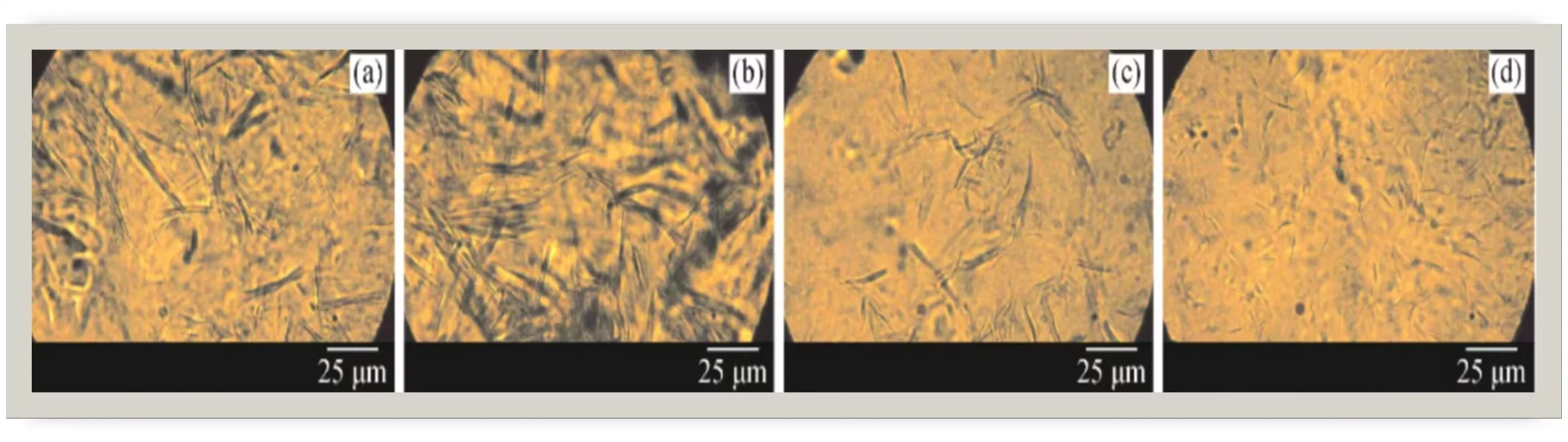
Figure 1. Wax deposition comparison before and after electromagnetic treatment.

Electromagnetic wax prevention system — technical parameters, installation requirements and well-screening criteria.

Speak directly with an engineer: [email protected] | WhatsApp on request.

References

[1] Sousa, A. M.; Ribeiro, T. P.; Pereira, M. J.; Matos, H. A. “Review of the Economic and Environmental Impacts of Producing Waxy Crude Oils.” *Energies* 2023, 16(1), 120. https://www.mdpi.com/1996-1073/16/1/120

[2] “Experimental study of the effects of a magnetic field / magnetic field-ferromagnetic nanocomposite pour point depressant on wax deposition.” *RSC Advances* 2024, 14(9), 6234–6245. https://pmc.ncbi.nlm.nih.gov/articles/PMC10875419/

[3] “The Effect of Magnetic Field on the Deposition of Paraffin Wax on the Oil Pipe.” *Advanced Materials Research* Vol. 788, pp. 719–723. https://www.scientific.net/AMR.788.719